Polygonal approximation of curves
www.kovalevsky.de, last update: October 26, 2011
 Let me know
what you think
| Home | Index of Lectures | << Prev | Next >> | PDF Version of this Page |
Polygonal approximation of curveswww.kovalevsky.de, last update: October 26, 2011 |
|
Let me know what you think |
|
|
Given is a digital curve C in a 2D image. We want to approximate C by a polygon which has as few as possible edges
and is "similar" to C. One of the possible criterions of the similarity is the Hausdorff distance:
Let S1
and S2 be two sets of points. Let us denote the distance between the points p and q
as
 |
 |
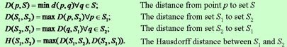
| Sample: All three small arrows have the length = 2. Here the Hausdorff distance between the black and the red curve is <2, however, the "true deviation" is much greater. Schlesinger has suggested a more adequate measure of the similarity of curves. |
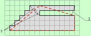
Given are two digital curves C1 and C2 . Take m points
along C1 and n points along C2. Thus one gets two ordered
sets M1 and M2 of points. The smaller the distance between subsequent
points the more precise the estimate of the similarity. Let us denote the distance between two points p and q as
Find the monotone map F: M1→M2, where monotone means that
for any two points p and q of M1 such that p > q also
F(p) > F(q) holds. The sign " > " in "p > q" means that the point p follows the point
q in the sequence M1.
We look for the smallest value of the maximum distance between the corresponding points.
This value is the Schlesinger distance
Schlesinger has also suggested an efficient algorithm for computing the distance DS for any two digital curves. The value of
DS for our example can be computed as follows. Let the black curve be B and the red one be R. They are subdivided
into corresponding segments
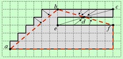 |
| The value of DS for the above example is defined by the length of |
The advantage of this method is that it is very simple to understand and to program. The idea is as follows. Given is the curve
C and the maximum allowed distance ε from the points of C to the polygon. Take an arbitrary point
P1 of C. Find the point P2 with the greatest distance from
P1. Now the curve is subdivided into two segments:
| An example with |
 |
| Split phase: Merge phase: |
The split-and-merge method is rather slow because each point must be tested many times, depending upon the number of splittings of
the segment to which it belongs. This method minimizes the Hausdorff distance, not the Schlesinger distance.
An efficient method called the sector method was suggested in the 70th by Williams. The idea is as follows:
1) Start with some point P1 of the curve C. Test all subsequent points. For each point
Pi with i>1 and
2) If the next point Pi (fig. P3 or
P4) lies in the sector, then a new circle with its center at Pi
and a sector S are constructed. The new sector is the intersection of S with the old one.
3) If the next point Pi (fig. P5) lies outside of the new sector,
then there is no straight line L through P1 and Pi such that
all points between P1 and Pi have a distance to L less
than ε. Therefore Pi cannot serve as a polygon edge. The point before
Pi
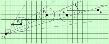 |
The sector method is fast because it tests each point only once. However, it guaranties only that the Hausdorff distance between the
curve and the polygon is less than the prescribed tolerance ε. The following additional condition for interrupting the
current segment of the curve,
that should be approximated by the current edge of the polygon, has been introduced. The point Pmax
of the current segment, which has the greatest distance from the starting point of the segment, must be defined during the processing
of the segment. If the projection of the actual point Pi onto the line
In the following example red points are those at which the algorithm comes to the decision to interrupt the current segment. The
tolerance ε = 1.5.
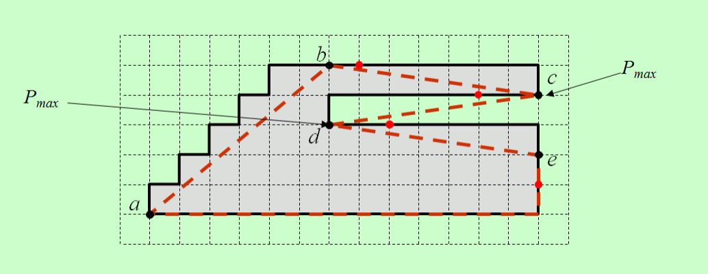 |
| An important drawback of the sector method is that it "cuts off" the vertices of right angles with sides parallel to the coordinate axes. The reason is that it only checks whether the distance of the given points from the polygon is less than the threshold. | 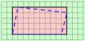 |
| A better method must also minimize the distance of the points from the polygon while retaining the number of polygon edges as small as possible. These contradictive requirements are expressed in the following minimization criterion: | 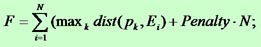 |
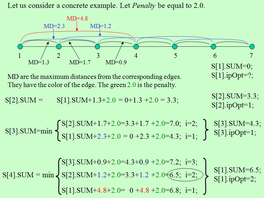
Here is N the number of the polygon edges, "Penalty" is a predefined constant,
dist(pk ,Ei) is the distance from the point
pk belonging to the ith segment of the curve to the edge Ei.
The maximum is with respect to all points of the ith segment.
The minimization problem can be solved by means of the dynamic programming in the following way. The curve (closed or open) is
represented as a sequence of points
| Let us draw the elements of | 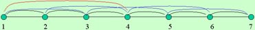 |
This method brings the best results as to the precision of the approximation. However, it must be still improved as to its time consuming. One of the ways of doing this consists in subdividing the given curve into longest DSSs and applying the optimization method to the endpoints of the DSSs. However, this approach needs some additional research to find a fast method of estimating the maximum deviation of the points of a DSS from the line connecting its end points. It is also necessary to eliminate DSSs looking like the following two:
 |
since they will give rise to the above mentioned problem of "cutting off" the vertices of right angles. The version explained above brings the optimal solution for a fixed starting point of the polygon. The non-trivial, fast solution for the optimal starting point must be still developed. Thus, there is still some research work to be done to bring this method to perfection. |
| top of page: |