Sub-pixel estiimation of the curvature

Sub-pixel estimation of curvature www.kovalevsky.de, last update: October 26, 2011		Let me know what you think
Digitization of regions with an approximately constant brightness Intersection of a regions boundary with a pair of adjacent pixels Intersection areas SA (small area) and GA (big area) as functions of t and α Recognition of the 6 cases by means of the areas SA and GA Solution of the equations in t and α defines a sub-pixel point for each pixel pair Example of the sub-pixel boundary of an ideal elliptic region and its curvature An example of calculating the curvature Conclusions References

Digitization of regions with an approximately constant brightness

A grid of pixels with a projection of an object
We consider [1] the pixels as small rectangles. This supposition is adequate if the light sensitive elementary devices (the CCD or CMOS cells) of the digitizing device, (a scanner or a digital camera) have rectangular apertures and the spaces between the apertures are negligible. Then the digitizing device assigns to a pixel a grey value proportional to the portion of the area of the corresponding rectangle covered by the light area.

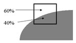An example: 0.6 of the pixel area is covered by the light area. Then the grey value is equal to
GV=Back + 0.6*(Fore−Back).
If Back== 20 and Fore== 255 then GV= 20+0.6*(255−20) = 161.

Intersection of a regions boundary with a pair of adjacent pixels

We consider a small part of region near its boundary as a half-plane.

Six cases of the intersection of a half-plane with a pair of pixels

The cases may be distinguished by the number of vertices of the resulting two polygons.
The green crosses x show the intersection points SP (sub-pixel point).
The parameter t is the distance indicated by the arrows.
The areas of the intersection SA (small area) and GA (big area) are defined in each of the cases by different functions of t and alpha.

Intersection areas SA (small area) and GA (big area) as functions of t and α

Case	SA	GA
0	0	t+0.5
1	t−0.5	1
2	0.5⋅L²⋅cot(α) with L=0.5+(t−0.5)⋅tan(α)	1.0−0.5⋅K²⋅cot(α) with K=0.5−(t−0.5)⋅tan(α)
3	0.5−(1.0−t)⋅tan(α)	0.5+t⋅tan(α)
4	SA=0.5−(1.0−t)⋅tan(α)	1.0−0.5⋅K²⋅cot(α) with K=0.5−(t−0.5)·tan(α)
5	0.5⋅L²⋅cot(α) with L=0.5+(t−0.5)⋅tan(α)	0.5+t⋅tan(α)

Recognition of the 6 cases by means of the areas SA and GA

The recognition algorithm:
If GA== 1 then case 1;
else if SA == 0 then case 0;
else if SA > max(GA/3, 3*(GA−3/4)+1/4) then case 3;
else if SA >= 4*(GA−0.5)² and GA < 3/4 then case 5;
else if SA > 0.5−0.5*sqrt(1−GA) and GA > 3/4 then case 4;
else case 2.

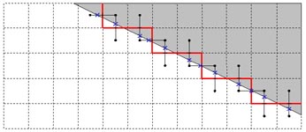Solution of the equations in t and α defines a sub-pixel point for each pixel pair

The boundary of a binarized image (the red solid line) with the sub-pixel points SP labeled by blue crosses. The threshold of the binarization lies in the middle between the maximum and minimum gray value.
Definition of the sub-pixel boundary SPB: The sub-pixel boundary of a region R in a gray value image (with no shading) is a polygon whose vertices are the sub-pixel points. An edge of the polygon connects each two sub-pixel points corresponding to subsequent boundary cracks.

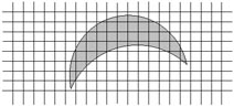
Example of the sub-pixel boundary of an ideal elliptic region and its curvature

Artificial elliptical area Curvature of the boundary
Maximum relative error = 0.71*10^-2/12.2*10^-2 = 6%

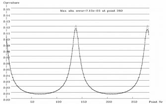The algorithm:

1. Trace the boundary of the region and store the sub-pixel points.
2. Smooth the coordinates of the points by a Gaussian filter with sigma ~= 4 points.
3. Compute the curvature at each sub-pixel point with a great chord (about 1/10 of the number of cracks in a closed curve) and store the results.
4. Read the points anew, estimate the second derivative of the curvature with respect to the arc length (as an estimate of F4 in (3) of the lecture "Curvature of curves"), choose for each point the optimal chord length: optim Δx = (48*ε/F4)^1/4 and recompute the curvature by means of the optimal chord.

An example of calculating the curvature

The gray value image of a link of a bicycle chain (taken by a digital camera)	The curvature of the outer boundary of the link Error about 4%

Conclusions

The reasons of the low precision of the most methods of estimating the curvature are the following:
1. The value of the curvature depends upon the second derivative of the coordinates of the points of the curve.
2. The precision of calculating derivatives depends dramatically on the precision of measuring the coordinates.
3. In a digital image the uncertainty of the coordinates is about 1 pixel and this amount strongly influences the derivatives.

To measure the curvature of the boundary of an approximately homogeneous subset S of a 2D image we suggest to use the gray values at the boundary of S to improve the precision of estimating the coordinates of the points of the boundary. We suggest a method of estimating the coordinates with a precision of about 1/100 of a pixel. This gives us the possibility to estimate the curvature with a higher precision.

References

[1] V. Kovalevsky, Curvature in Digital 2D Images, International Journal of Pattern Recognition and Artificial Intelligence, vol. 15, No. 7, 2001, pp. 1183 - 1200.

You can download the paper [1] at The paper

Download: Print version

top of page:

Sub-pixel estimation of curvature