Segmentation and Binarization
www.kovalevsky.de, last update: October 26, 2011
 Let me know
what you think
| Home | Index of Lectures | << Prev | Next >> | PDF Version of this Page |
Segmentation and Binarizationwww.kovalevsky.de, last update: October 26, 2011 |
|
Let me know what you think |
|
|
The commonly used method of thresholding grey level images consists in using the grey value corresponding to the histogram minimum
as the threshold. The justification: the histogram of an image with two regions each having a constant grey level looks like two
columns. If noise is present, the histogram looks like two hills with a valley in-between.
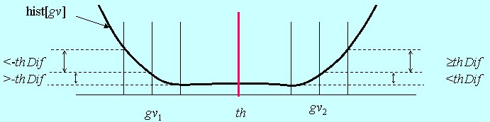
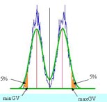 | The optimal threshold corresponds to the local minimum of the histogram, but not always to the global minimum. Therefore, it is necessary to restrict the area of the search for the minimum as to guaranty that at least some predefined portion of the image be black or white. For example, if you want that at least 5% of the image area is black, than you must find such a grey value minGV that 5% of the histogram area be to the left of minGV. Only minima to the right of minGV must be considered. Similarly, the choice of maxGV can guaranty that at least the desired portion of the area is white. |
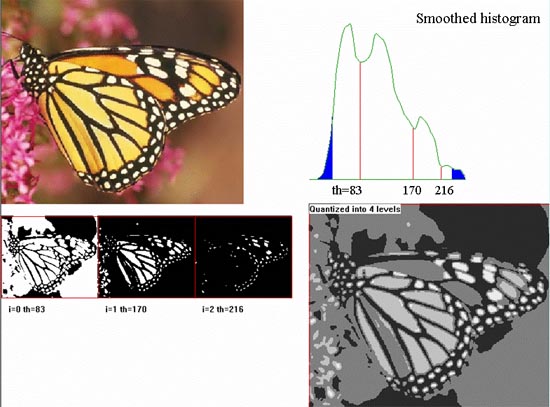 | Sometimes the histogram has more than one local minimum and the deepest one is not always the one corresponding to your desire. Then it is appropriate to display binary images for the thresholds corresponding to all mimima and choose the best one. Another possibility is to produce a multi-level image, each level corresponding to a space between two thresholds. Also levels corresponding to the grey values less than the first and greater than the last threshold must be provided. To make the search for minima more certain, it is necessary to smooth the histogram. |
Some images to be binarized have a strong shading, which means that the local average brightness changes gradually from one part of the image to another. If the light side of the darker area is brighter than the dark side of the light area then there exists no threshold separating these two areas.
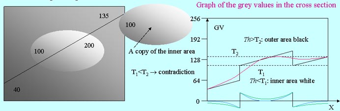 |
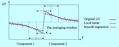
In such cases a shading correction can be useful: it is necessary to subtract the average grey value computed in a relatively large
window from all grey values of the image. The width of the window can be e.g. 1/3 of the width of the image. The fast averaging filter
can compute the average very fast. The blue line in the above figure shows the results of the subtraction in the case when the
averaging window was too small; the green line - in the case of a window being large enough. The window must be so large, that it
cannot be completely contained in some white AND in some black region. Otherwise the average becomes equal to the grey values in two
regions of different colors and the separation is impossible.
The difference between the original and the average grey levels may lie in the interval from -255 to +255. To compute the histogram
of the differences a bias of 256 must be added to the difference (since the index of an array in C++ must be non-negative). The
histogram must have 512 elements (while many of them are equal to zero).
The algorithm finds in this histogram the values of minGV and maxGV as explained above. In this case these values lie
between 0 and 510. Then the algorithm converts the differences into a usual grey level image with 256 levels by simply setting the
biased differences which are less than minGV equal to zero and those greater than
The value of thDif must be chosen in
 |
Definition (Pavlidis, 1977): The segmentation of an image I according to a given homogeneity predicate P is a
decomposition of I in disjoint non-empty subsets
1. The union of all Si is equal to I.
2. Each Si is connected.
3. The homogeneity predicate P is true for each Si.
4. It is false for the union of any number of adjacent subsets Si.
 | Examples of homogeneity predicates:
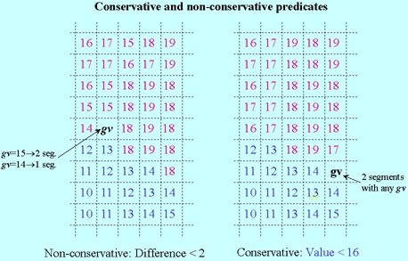
Two pixels are called directly equivalent if they have a common side and their grey values differ no more than by a
predefined value V. Let E be the transitive hull of the direct equivalence. The predicate P is true for a
subset S if all pixels of S are equivalent with respect to E. The predicate P thus defined has an important drawback: two adjacent segments S1 and S2 defined by means of P can merge together if we change the gray value of a single pixel at the common boundary of S1 and S2. A "good" predicate G must be conservative. This means, that if a set S is homogeneous with respect to G then each subset of S must be also homogeneous with respect to G. An example of a conservative predicate: a set S is homogeneous if the grey values of all pixels of S are less or equal to a given value V. |
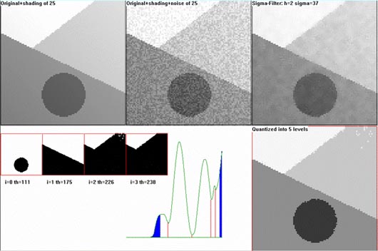 | Thresholding: works
well when there is no large shading and no strong noise. It is not expedient to test a segmentation method on some natural images because the correct segmentation of such an image is mostly unknown. A good test is on an artificial image produced of a well segmented image by adding some shading and noise to it. The thresholding program smoothes the image by the sigma-filter, calculates all local minima of the smoothed histogram and makes a quantized image. |
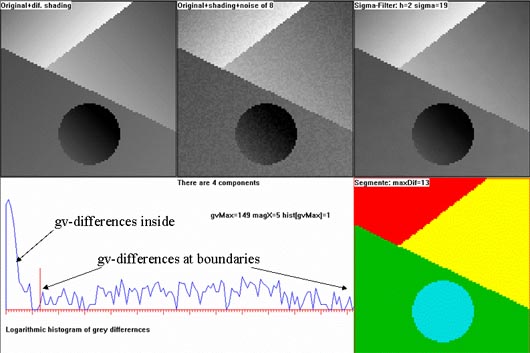 | Labeling connected
components with limited grey value differences This method is applicable even in the cases of arbitrarily oriented gradients of the shading in different segments. The shading and the noise must be not too strong so that after the filtering with the sigma-filter the gv-differences inside the segments are less than the differences at the segment boundaries. |
One difficult problem arises due to small grey level differences at the boundaries of the segments: two adjacent segments can merge
together if there is a single pair of adjacent pixels belonging to different segments and having a small grey difference.
To overcome this difficulty the following problem should be solved:
Given a grey value image GV(x,y), its temporary subdivision into connected components and a positive constant K
find for each component the "smooth" image
Z(x,y) satisfying the following condition:
The loss function LF contains two terms. The first term is the sum of the squared deviations of Z from GV.
It characterizes the precision of the approximation of GV by Z. The second term is the sum of the squares of the second
differences (a generalization of the second derivative for digital functions) of Z(x,y). It characterizes the
non-smoothness of Z; it increases with the local curvature of the surface Z(x,y). Due to the minimization of the
weighted sum of these two terms (with the weights equal to 1 and K) a compromise between the imprecision and the non-smoothness
of Z should be found. The minimization takes place with respect to all possible values of Z(x,y). The optimal
function Z(x,y) is called the "smooth regression" of GV(x,y) in a given component of the image.
This is a means for noise suppression which is better than a filter, since it considers the relative location of the pixels, while a
filter considers only their grey values.
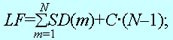 | Subdivide the image into connected components so that the loss function LF be minimal,
where SD(m) is the squared deviation of the gray values from the smooth regression of the mth component; C is a predefined constant "penalty for too many components"; N is the number of the components. |
| The difference between the smooth regression SR and the local mean |
 |
| The shape of the kernel depending upon the distance from the boundary |
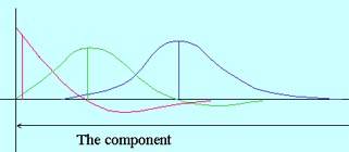 |
The problem for two-dimensional images must be yet solved. SR is again a convolution of GV(x,y) with some two-dimensional kernel, which is different for different pixels of the image, depending upon the distance of the pixel from the boundary and of the shape of the boundary of the component. The letter dependence make the problem difficult.
Download: Print version| :top of page |