Tracing Boundaries in 2D Images
 |
 |
 |
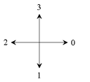
| coordinate system |
directions of the
Crack Code |
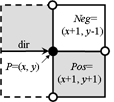
2 pixels Pos and Neg
must be tested |
The tracing is performed in combinatorial coordinates. The program goes from one boundary point to the next one along the boundary
cracks. To recognize the next boundary crack the program tests two pixels "Pos" and "Neg" lying ahead of the
actual crack. The program calculates the coordinates of these pixels by adding the 2D vectors "Positive[direction]"
and "Negative[direction]" to the vector "P" of the actual point. The vectors are predefined as small constant
arrays. Then the program gets the gray values (or colors) of the pixels from the given image while transforming the combinatorial
coordinates "Pos" and "Neg" to standard coordinates by simply dividing them by 2 (integer division).
The direction of the next crack is then calculated depending on the two gray values simply by adding a 1 or a 3 modulo 4 to the
actual direction. Then the actual point moves along the new direction. The process stops when the starting point is reached again.
The algorithm in pseudo-code:
P.X=Start.X; P.Y=Start.Y; direction=1; // P is the current point
do
{ Pos=P+Positive[direction];         // Pos is the positive pixel
  Neg=P+Negative[direction];         // Neg is the negative pixel
  if (image[Pos/2]==foreground)      // Pos/2 is in standard raster
    direction=(direction+1) MOD 4;   // positive turn
  else
    if (image[Neg/2]==background)    // Neg/2 is in standard raster
      direction=(direction+3) MOD 4; // negative turn
  P=P+step[direction];               // a move in the new direction
} while( P.X!=Start.X || P.Y!=Start.Y);
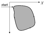
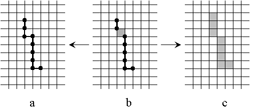
Searching a Starting Point of Tracing
For finding a starting point of the tracing the image must be scanned raw by raw. As soon as two subsequent pixels of different colors are found the starting point is defined as the upper end point of the crack lying between the pixels.
 |
The foreground object remains on the negative side of tracing.
To avoid multiple tracing the already visited vertical cracks must be labeled. The algorithm is slightly simpler if it has to start
only at a transition from the background to the foreground but not at a transition from the foreground to the background. |
The Code of "Trace" in native C language
Simple C and C++ have no structure like class CPoint which may be used as a 2D vector with addition. Therefore we use in the "Console" integer variables as components of a vector. The addition of vectors must be done component by component.
#define US unsigned char
int POSX[4]={1,-1,-1, 1}; // move from point to positive pixel
int POSY[4]={1, 1,-1,-1};
int NEGX[4]={1, 1,-1,-1}; // move from point to negative pixel
int NEGY[4]={-1,1, 1,-1};
int StepX[4]={2,0,-2, 0}; // move to next point
int StepY[4]={0,2, 0,-2};

int Value( US *img, int NX, int NY, int xc, int yc )
{ if( xc>=0 && xc<2*NX && yc>=0 && yc<2*NY ) return img[yc/2*NX+xc/2];
  return 0; // the function returns the value of the cell (xc, yc)
}
int Label( US *img, int NX, int NY, int xc, int yc )
{ if ( (xc&1)+(yc&1)!=1 )
  { printf( "Label: (%d,%d) is no crack. Stop\n",xc,yc ); return -1; }
  if ( xc<0 )
  { printf( "Bad coordinate xc=%d. Stop\n", xc );   return -1; }
  img[yc/2*NX+xc/2]|=VERT;  // labeling a vertical crack
  return 1;
}
int Trace( US *img, int NX, int NY, int xc, int yc )
{ int cnt=0, deb=1, rv=1, x=xc, y=yc, dir=1;
  do  // (x, y) is the current point; (PosX, PosY) and (NegX, NegY) are pixels
  { int PosX=x+POSX[dir];     int PosY=y+POSY[dir];
    int NegX=x+NEGX[dir];     int NegY=y+NEGY[dir];
    int ValPos=Value( img, NX, NY, PosX, PosY ); // value of img[Pos]
    int ValNeg=Value( img, NX, NY, NegX, NegY ); // value of img[Neg]
    if      (ValPos >0) dir = (dir+1)%4;         // positive turn
    else if (ValNeg==0) dir = (dir+3)%4;         // negative turn
    if ( dir==1 ) rv=Label(img,NX,NY,x,y+1);
  //if ( dir==3 ) rv=Label(img,NX,NY,x,y-1);
    if ( rv<0 ) { printf( "Error at cnt=%d\n",cnt ); return -1; }
    x = x+StepX[dir];  y=y+StepY[dir];
    cnt++;
  } while( (x!=xc || y!=yc) && cnt<1000 );
  return cnt;
}

 |
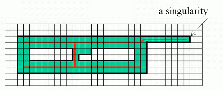
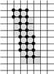
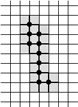
Image Reconstruction by Filling the Interiors of Boundaries
To check whether an n-cell P of an n-space lies in the interior of an (n-1)-dimensional manifold
M it is sufficient to count the intersections of M with a ray (e.g. parallel to X coordinate axis) going from P to the border of the space.
The counting is easy to perform only if the space is a complex. Otherwise it is difficult to distinguish between intersection and
tangency.
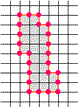
If the curve is given as a sequence of pixels then one needs to investigate three raws of the image to distinguish between crossing
and tangency. Indeed, in the figures "intersection" and "tangency" the third raw is exactly the same.
However, when representing the image as a complex a curve becomes a sequence of alternating 0- and 1-cells. Now the mentioned
problem becomes easy since a ray consisting of pixels and vertical cracks between them can only cross a curve at a vertical crack.
A tangency is impossible.
The algorithm of filling is now very simple: before starting the filling all vertical cracks of the curve must be labeled
(in some way) in the image. In the case of an nD image the (n−1)-dimensional cells orthogonal to the chosen
coordinate axis must be labeled. The program scans the image raw by raw. It sets the logical variable fill
to FALSE
at the beginning of each raw. As soon as a labeled vertical crack (an (n−1)-cell) is encountered the variable
fill is inverted: fill=NOT fill. If fill
is TRUE the next pixel (n-cell) gets the label of the foreground, otherwise - the label of the background.
 |
 |
 |
| intersection |
tangency |
no problem in a complex |
The pseudocode (tested for n=2,3,4):
Choose a coordinate axis of the Cartesian space, e.g. the X-axis. Label all (n-1)-cells of M whose normal is
parallel to X.
for ( each row R parallel to X )
{ fill=FALSE;
  for ( each n-cell C in the row R )
    { if ( the first (n-1)-side of C is labeled ) fill = NOT fill;
      if ( fill==TRUE ) C = foreground;
      else              C = background;
    }
}
This algorithm with some small changes is applicable also in higher dimensions.
Component Labeling in an n-dimensional Space
The space is represented as an n-dimensional array S. The indices correspond to the coordinates. Each element of S contains a color. After the labeling each element of S gets (in another array L) the label of the component which it belongs to.
 |
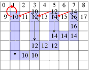 |
The naive approach:
About NY3/2 rewritings |
The advanced approach:
About NX/2 rewritings |
Labeling Connected Components:
Given is a segmented nD image: the principal cells (i.e. the n-cells) have a relatively small number of colors.
Otherwise it may happen that each pixel of a colored image is a connected component. The problem consists in finding the maximal
connected subsets of the image, each subset containing principal cells of a constant color. Then it is necessary to number the
components and to assign to each principal cell the label containing the number of its component. The labels are saved in an auxiliary
array L.
The naive approach consists in scanning the image raw by raw and assigning to each pixel that has no adjacent pixels of the same color
in the already scanned subset the next unused label. If the next pixel has adjacent pixels of the same color and they have different
labels then the smallest of the labels is assigned to the pixel and all other encountered label must be replaced by the smallest one.
The replacement may affect in the worst case up to NY 2/2 pixels where NY is the number of rows in the image.
The total number of replacements may then be of the order of NY 3/2.
The suggested method (Galler and Fischer, 1964) is based on the following idea. We explain the method for the 2D case, but it is
applicable for any dimension. The label of a component must be such that it is possible to find the address in the memory of some
definite pixel called the root of the component, when starting from the label. At the start of the program each pixel
(x, y) of the array L of labels gets the index x+NX*y as its label where NX is the number of columns of the image.
Thus at start each pixel is considered as a component and it is the root of the component.
The program scans the image raw by raw. If the next pixel P has adjacent pixels of the same color among the already visited
pixels and they have different labels then the smallest root label is assigned to P and to the roots of all encountered pixels.
Thus all components that meet at the running pixel get the same root. Thus they become merged to a single component. The labels of
pixels that are no roots remain unchanged. The replacement may affect in the above mentioned worst case only NX/2 pixels.
After the first scan each pixel contains the root label of its component. During the second scan the labels are replaced by
subsequent integer numbers.
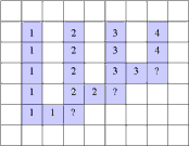
A Simple Example of Labeling :
 |
 |
The algorithm scans the image two times: after the first run each element gets in L the "root" of its component as its label. During the second run the roots are replaced by subsequent numbers. |
| first run | second run | |
The pseudo-code:
A second array L of the same size as S must be allocated. Each element of L must contain at least log2|S|
bits where NS is the number of elements of S.
for (i=0; i<|S|; i++) L[i]=i;

for (i=0; i<|S|; i++)
{ for (j=0; j Max_n]; j++)    // "Max_n" is the maximum number of already visited adjacent elements
  { k=Neighbour(i, j);       // "Neighbour(i, j)" the jth adjacent element of "i"
    if (Adjacent(i, k) AND S[k]==S[i]) SetEquivalent(i, k, L);
  }
}
SecondRun(L, |S|);

void SetEquivalent(i, k, L)
{ if (Root(i, L)>Root(k, L) ) L[Root(k, L)]=Root(i, L);
  else                        L[Root(i, L)]=Root(k, L);
}

int Root(k, L)
{ for(int i=0; i<|L|; i++)
  { if (k==L[k]) return k;
    k=L[k];
  }
  ErrorMessage( ); return -1;
}

void SecondRun(L, N)
{ for (int i = 0, int count=1; i<=N-1; i++)
  { int label=L[i];
    if (label==i ) { L[i]=count;  count++;}
    else             L[i]=L[label];
  }
}
We present in this section a method of producing skeletons from pictures represented as 2D or 3D cell complexes because we need cells of lower dimensions (the points and the cracks in the 2D case).
Let us start with the definition.
Definition of a Skeleton
The skeleton of a given set T of an n-dimensional (n=2,3) image I is a subset
S⊂T with the following properties:
a) S has the same number of connected components as T;
b) The number of connected components of I−S is the same as that of I−T;
c) Certain singularities of T are retained in S;
d) S is the smallest subset of T having the properties a) to c).
 | |
Singularities may be defined e.g. as the "end points" in a 2D image or "borders of layers" in a 3D image etc. |
The problem consists in finding the conditions under which a cell of the foreground T may be deleted, i.e. reassigned to the
background B=I−T without changing the number of the components of both T and B.
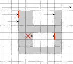
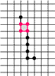
Parallel Calculation of the Skaeleton
A well-known difficulty in calculating skeletons by a parallel algorithm is demonstrated in the figure: Each of the marked pixels
can be removed without violating the above conditions but not both of them simultaneously.
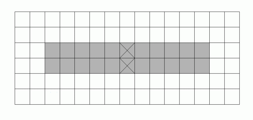 |
This makes the parallel calculation of a skeleton to a difficult problem.
|
To solve the problem we consider the notion of the incidence structure of a cell.
The Incidence Structure of a Cell
A complex IS(C, I)=SON(C, I) ∪ Cl(C, I)−{C} is called the incidence structure
of the cell C relative to
the n-space I. It is the complex consisting of all cells incident to the cell C excluding C itself.
We shall denote the incidence structure by IS.
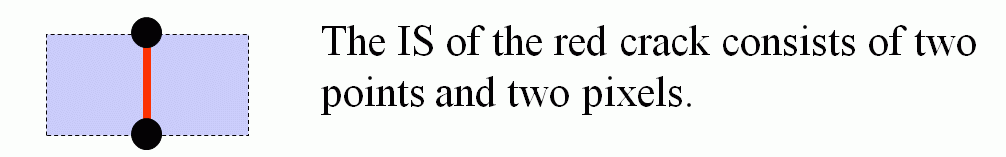
An Example:
IS-simple Cells
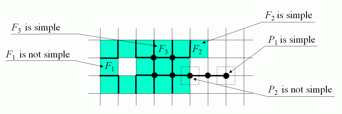 | |
| The membership of a cell C of any dimension may be changed between the foreground T and the background B if
each of the intersections IS(C,I)∩T and IS(C,I)∩B are not empty and
connected.
Such a cell is called IS-simple relative to the set T or simple.In an n-dimensional space the condition is
a little more complicated: each of the intersections must be a single (n−1)-dimensional topological ball.
|
The Algorithm
The algorithm consists in deleting simple cells alternately from the closing and open boundary of the foreground subset being
processed. Cells considered as singularities are not deleted. Singularities may be defined e.g. as endpoints of lines in the
two-dimensional case or as boundaries of "flat cakes"
in the three-dimensional case.
 | |
The skeleton S thus constructed may contain both principal cells and cells of lower dimensions (b). However, it is
easily possible to transform it either to a "thin skeleton" consisting of cells of dimension less or equal
to n−1 (a) or to a "thick skeleton" (b) consisting of principal cells and a minimum number of other
cells that are necessary to make the components of S connected. |
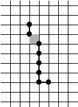
Example of Computing the Skeleton of a Region in 2D
| The region S |
Its frontier
B=Fr(S) |
C=S−Simple(B) |
O=OB(C) |
F=C−Simple(O) |
Skel=F−Simple(Fr(F)) |
 |
 |
 |
 |
 |
 |
Example of a 3D Skeleton