The author has developed three algorithms for economical and exact encoding of surfaces in 3D spaces. He has compared them with the
algorithm known as "Depth-First Search" of a graph.
Depth-First Search
It is well-known that the set of the facets of a surface can be considered as a graph: facets are the vertices and any two adjacent
facets are connected by an edge of the graph. The aim of the algorithm is to put all facets of the surface into a list. If a facet
is adjacent to that previously put into the list, then only the differences of coordinates are saved in the list. Otherwise
coordinates are saved. The algorithm starts with an arbitrary facet, puts it into the stack
("last in first out") and starts a while-loop which is running while the stack is not empty. In the loop a facet F is being
popped form the stack. If it is not labeled as being already in the list then it is put into the list and labeled..
Then all facets adjacent to F are put into the stack. This algorithm is rather simple and fast, but it is not
economical: It needs on an average 2.5 bytes per facet even if sequences of adjacent facets are coded by differences of coordinates.
The sequences are mostly too short.
Euler Circuit
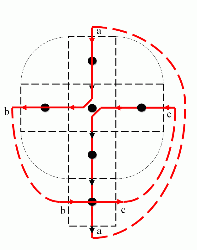
The author has developed an algorithm which finds the Euler circuit of the adjacency graph of the facets. The algorithm uses a
directed graph (digraph) with the aim to make the number of edges as small as possible. The Euler circuit is a closed sequence
of facets and the 0- or 1-cells in between containing each 0- or 1-cell only once (a facet can be contained twice). The Euler
circuit can be encoded very economically by the differences of the coordinates of two adjacent facets. Experiments have showed
that this code needs on an average about 0.75 bytes per facet.
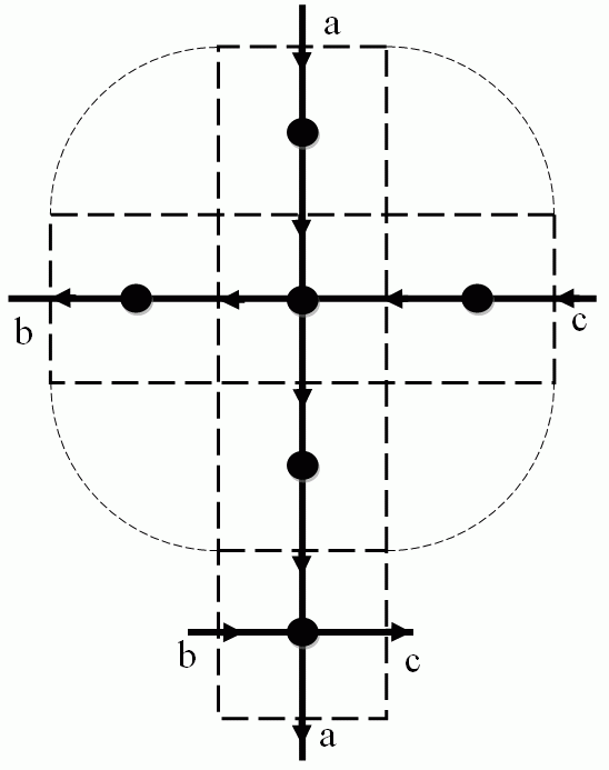
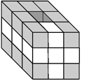
| Digraph of the adjacencies in the surface of a small cube | |
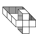
Euler circuit of the surface of a small cube |
 | |
 |
Spiral Tracing
This algorithm takes an arbitrary facet of the surface S as a starting one and labels its closure. This is the "germ-cell" of the
set L of the labeled facets. The algorithm traces the opening boundary (see lecture "Introduction") of L and labels
all "simple" facets. A facet is simple if the intersection of its boundary with the boundary of L is not empty and connected
while the intersection of its boundary with the complement of L is also not empty. The trace looks like a spiral. This method
is less efficient than that of Euler circuit: it needs between 1.0 and 2.0 bytes per facet depending on the number of tunnels in
the surface. It is, however, interesting since it defines the genus (number of tunnels) of the surface.
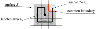 | |
The idea of the tracing:
The set L of labeled simple facets remains always topologically equivalent to a disk (a 2-ball). |
| Example of tracing |
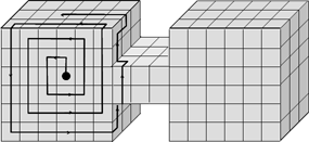 |
Recognition of the Genus of the Surface
The set of simple facets (grey) composes
a topological disk (2-ball) |
|
The set of remaining non-simple cells (white)
carries information abou the genus. |
 | |
 |
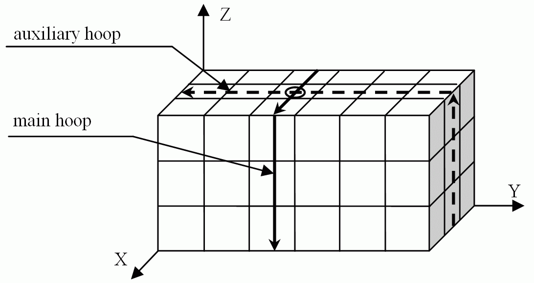
Economical Hoop Code
This is the most economical method. It finds and traces facets lying in the boundary of a two-dimensional slice of the body
(solid line in the figure below).
This boundary is called a "hoop". Another "auxiliary hoop" (dashed line) is used for finding the starting facets of the main hoops.
It is sufficient to save the coordinates of a single starting facet of a hoop. For all other
facets only the differences of their coordinates are encoded. The efficiency of this method is between 0.21 and 0.5 byte per
facet for bodies whose surface has no singularities. However, for bodies with singular surfaces the efficiency can be rather bad.
This is the main drawback of this method.
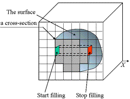
Exact Reconstruction of Images by Filling the Interiors of Surfaces in 3D
The algorithm is similar to that presented in Lecture 2 for filling interiors of curves in 2D. It is necessary to label the
facets (2-cells) of the given surface whose normals are parallel (or anti-parallel) to one of the coordinate axes. Then the
algorithms scans all rows of the grid, that are parallel to the chosen axis, and counts the labeled facets. The filling begins
at each odd count and ends at each even count. This algorithm can exacltly reconstruct the 3D image from the codes of the surfaces.
| The surface | The pseudocode |
 |
Choose a coordinate axis of the Cartesian space, e.g. the X-axis.
Label all (n−1)-cells of M whose normal is parallel to X.
for ( each row R parallel to X )
{ fill=FALSE;
  for ( each n-cell C in the row R )
  { if ( the 1st (n-1)-side of C is labeled )
      fill = NOT fill;
    if ( fill==TRUE ) C = foreground;
    else              C = background;
  }
}
|
[1] V. Kovalevsky, A Topological Method of Surface Representation, In: Bertrand, G. et all (eds.),
Lecture Notes in Computer Science, vol. 1568, Springer 1999, pp. 118-135.
[2] V. Kovalevsky: Geometry of Locally Finite Spaces, Monograph, Berlin 2008.
If you are interested in details see the reference [1]
and take the book: 'Geometry of Locally Finite Spaces'.
Download: Print version
Last update: October 24, 2011
 Depth First Search